Introduction
 Source: CalCOFI
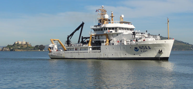
The California Cooperative Oceanic Fisheries Investigations (CalCOFI) is an organization that focuses on studying the marine environment surrounding the California coast in order to investigate the relationships between climate, fish population, and other human activities.
Our project initially focused on two separate datasets:
Fish Larvae Catch Data
This data was collected from CalCOFI cruises and was used to measure quantities and catch amounts of 6 different fish species.
# rename columns to non-scientific names for readability
larval = larval_df.rename(columns={'Engraulis.mordax':'Anchovy, Northern','Trachurus.symmetricus':'Mackerel, Jack', 'Scomber.japonicus':'Mackerel, Pacific','Lampridiformes1':'Opah','Sardinops.sagax':'Sardine','Seriola.lalandi':'Yellowtail'})

# select columns to show
cols_to_display_larval = ['longitude','latitude','year','season','Anchovy, Northern','Mackerel, Jack',
'Mackerel, Pacific','Opah','Sardine','Yellowtail']

# print head of selected columns
larval[cols_to_display_larval].head(10)
| longitude | latitude | year | season | Anchovy, Northern | Mackerel, Jack | Mackerel, Pacific | Opah | Sardine | Yellowtail | |
|---|---|---|---|---|---|---|---|---|---|---|
| 0 | -120.776667 | 35.086667 | 2019 | spring | 0.000000 | 0.0 | 0.0 | 0.0 | 0.0 | 0.0 |
| 1 | -120.915000 | 35.021667 | 2019 | spring | 0.000000 | 0.0 | 0.0 | 0.0 | 0.0 | 0.0 |
| 2 | -121.196667 | 34.890000 | 2019 | spring | 36.666667 | 0.0 | 0.0 | 0.0 | 0.0 | 0.0 |
| 3 | -121.551667 | 34.720000 | 2019 | spring | 40.720000 | 0.0 | 0.0 | 0.0 | 0.0 | 0.0 |
| 4 | -122.245000 | 34.390000 | 2019 | spring | 4.850000 | 0.0 | 0.0 | 0.0 | 0.0 | 0.0 |
| 5 | -122.958333 | 34.048333 | 2019 | spring | 4.340000 | 0.0 | 0.0 | 0.0 | 0.0 | 0.0 |
| 6 | -120.495000 | 34.465000 | 2019 | spring | 0.000000 | 0.0 | 0.0 | 0.0 | 0.0 | 0.0 |
| 7 | -120.528333 | 34.453333 | 2019 | spring | 4.170000 | 0.0 | 0.0 | 0.0 | 0.0 | 0.0 |
| 8 | -120.790000 | 34.328333 | 2019 | spring | 1801.358491 | 0.0 | 0.0 | 0.0 | 0.0 | 0.0 |
| 9 | -121.153333 | 34.150000 | 2019 | spring | 351.909091 | 0.0 | 0.0 | 0.0 | 0.0 | 0.0 |
The larvae catch dataset contains information on time (year),location (latitude/longitude), and the amount (pounds) of larvae found. It is sorted by species type.
The dataset is very sparse, since the majority of cruises caught zero pounds of a given larvae species. Scroll through and see just how many types of fish there are, and how few are caught per cruise!
Commercial Fish Data
This data was collected from various California fisheries and was used to supplement the fish catch data by providing additional information on amounts of fish caught.
# remove NAs from fishery data
cleaned_fishery = fishery_updated.dropna(how='any')
cleaned_fishery = cleaned_fishery[cleaned_fishery['Total Price'] != ' ']

# print data
cleaned_fishery.head(10)
| Year | Quarter | GroupBlocks | Species ID | Species Name | Pounds | Total Price | |
|---|---|---|---|---|---|---|---|
| 0 | 1987 | Qtr 1 | 1032.0 | 40.0 | Yellowtail | 256.0 | $272 |
| 3 | 1987 | Qtr 2 | 1032.0 | 40.0 | Yellowtail | 1710.0 | $1,511 |
| 5 | 1987 | Qtr 2 | 1034.0 | 40.0 | Yellowtail | 1417.0 | $1,177 |
| 6 | 1987 | Qtr 2 | 1035.0 | 40.0 | Yellowtail | 6457.0 | $6,267 |
| 8 | 1987 | Qtr 2 | 600.0 | 40.0 | Yellowtail | 3071.0 | $2,644 |
| 9 | 1987 | Qtr 2 | 700.0 | 40.0 | Yellowtail | 2622.0 | $2,549 |
| 10 | 1987 | Qtr 2 | 800.0 | 40.0 | Yellowtail | 2815.0 | $2,704 |
| 11 | 1987 | Qtr 3 | 1032.0 | 40.0 | Yellowtail | 7335.0 | $8,019 |
| 13 | 1987 | Qtr 3 | 1034.0 | 40.0 | Yellowtail | 3645.0 | $3,127 |
| 14 | 1987 | Qtr 3 | 1035.0 | 40.0 | Yellowtail | 4458.0 | $4,397 |
The commercial fishery dataset contains information on time (year/month), location (latitude/longitude), amount of fish caught (pounds), and price-per-pound (dollars) of each fish in every given catch year.
Due to data privacy rules, some of the information relating to price-per-pound and pounds caught are redacted.
In the beginning, we explored these two datasets with the intention of finding a relationship between the amount of fish larvae detected and the amount of adult fish caught. Over time, our workflow and goal became more developed, leading us to incorporate a third dataset into our project:
Bottle and Cast Data
This dataset was used to incorporate additional environmental factors with our larvae and commercial fish data.
# rename columns for readability
bottle_preview = bottle.rename(
    columns={
        'Cst_Cnt':'Cast Count',
        'Ocean degC':'Water Temperature (C)',
        'Salnty':'Water Salinity'}
    )

# select columns to keep
bottle_preview[['Year','Cast Count','Water Temperature (C)','Water Salinity']].head(10)
| Year | Cast Count | Water Temperature (C) | Water Salinity | |
|---|---|---|---|---|
| 0 | 1949 | 462.984846 | 9.008097 | 33.875273 |
| 1 | 1950 | 1481.434568 | 8.670928 | 33.884616 |
| 2 | 1951 | 2938.570895 | 8.544260 | 33.874098 |
| 3 | 1952 | 4422.839220 | 9.408110 | 33.753253 |
| 4 | 1953 | 5845.616774 | 9.794919 | 33.796447 |
| 5 | 1954 | 6875.716300 | 9.762641 | 33.773640 |
| 6 | 1955 | 7645.020691 | 9.516349 | 33.854505 |
| 7 | 1956 | 8329.149738 | 9.246048 | 33.844304 |
| 8 | 1957 | 9043.949093 | 10.520039 | 33.798667 |
| 9 | 1958 | 9883.231321 | 10.693563 | 33.767853 |
The bottle and cast data contains information on cast counts, water temperature (celcius) during a given cast, and water salinity (salinity scale).
Cast refers to information about the cruise itself, while bottle refers to information regarding the water quality, such as temperature and salinity.
After incorporating the bottle and cast dataset, our project’s goal shifted from establishing whether any correlations can be drawn from the fish larvae and fish catch to investigating any environmental factors that may add variance to the relationship as well. Additionally, it helped us focus on one species in particular: the Pacific Sardine.
The Shift Towards Sardine
# clean and process landing data (time series version)
fish_count_ts_df = landing_summary_ts.filter(['Year','SpeciesName'],axis=1)
fish_count_ts_df.drop(fish_count_ts_df.tail(5).index,inplace=True)

# create separate dataframes for each species
# groupby year, find counts per year, and rename columns
mjack_ts = fish_count_ts_df[fish_count_ts_df['SpeciesName']=='Mackerel, jack'].groupby('Year').count().reset_index().rename(columns={'SpeciesName':'Count'})
anchovy_ts = fish_count_ts_df[fish_count_ts_df['SpeciesName']=='Anchovy, northern             '].groupby('Year').count().reset_index().rename(columns={'SpeciesName':'Count'})
mpacific_ts = fish_count_ts_df[fish_count_ts_df['SpeciesName']=='Mackerel, Pacific'].groupby('Year').count().reset_index().rename(columns={'SpeciesName':'Count'})
yellowtail_ts = fish_count_ts_df[fish_count_ts_df['SpeciesName']=='Yellowtail'].groupby('Year').count().reset_index().rename(columns={'SpeciesName':'Count'})
opah_ts = fish_count_ts_df[fish_count_ts_df['SpeciesName']=='Opah'].groupby('Year').count().reset_index().rename(columns={'SpeciesName':'Count'})
sardine_ts2 = fish_count_ts_df[fish_count_ts_df['SpeciesName']=='Sardine, Pacific              '].groupby('Year').count().reset_index().rename(columns={'SpeciesName':'Count'})

# label each dataframe based on species type
mjack_ts['Species'] = 'Mackerel Jack'
anchovy_ts['Species'] = 'Anchovy'
mpacific_ts['Species'] = 'Mackerel Pacific'
yellowtail_ts['Species'] = 'Yellowtail'
opah_ts['Species'] = 'Opah'
sardine_ts2['Species'] = 'Sardine'

# combine dataframes
species_ts = pd.concat([mjack_ts,anchovy_ts,mpacific_ts,yellowtail_ts,opah_ts,sardine_ts2],ignore_index=True)

# pivot combined dataframe
species_total_ts = species_ts.pivot(
    index = 'Year',
    columns = 'Species',
    values = 'Count'
)

# impute missing values in Opah column with means
species_total_ts_final = species_total_ts.fillna(round(species_total_ts.Opah.mean(),1))

# construct line plot
# add custom colors to grey out all species except sardine
fig_species_total = px.line(
    species_total_ts_final,
    y = ['Sardine','Anchovy','Mackerel Jack','Mackerel Pacific', 'Opah', 'Yellowtail'],
    color_discrete_sequence= ['blue','gray','gray','gray','gray','gray'],
    labels = {'value':'Abundance (thousands)'},
    title = 'Abundance By Year (All Species)'
)

# add annotations to specified points on the lines
fig_species_total.update_layout(
    annotations=[
        {'x':8,'y':360,'text':'Mackerel Jack'},
        {'x':6,'y':268,'text':'Anchovy'},
        {'x':12,'y':438,'text':'Mackerel Pacific'},
        {'x':15,'y':264,'text':'Opah'},
        {'x':4,'y':144,'text':'Yellowtail'},
        {'x':38,'y':296,'text':'Sardine'}],
        showlegend=False)


fig_species_total.show()
While our datasets contain information on 6 different fish species, we decided to focus this project primarily on Sardinops sagax, or more commonly known as Pacific Sardine. We chose Sardine because differences in fish species characteristics, such as migration patterns or mating behaviors, made it difficult to identify patterns that apply to all of the species as a whole. Rather than focus on the behavior of all species as a whole, we aimed to find one specific species to center our analysis around- the Pacific Sardine.
Our choice was also influenced by the large amount of data we had on Sardines- more data will help us perform a more accurate analysis. Additionally, sardine is also the focus of the CalCOFI organization, which was originally formed to study the ecological consequences of a declining sardine population off the California coast. Although CalCOFI has now shifted its focus to studying the marine environment off the California coast as a whole, we decided that interesting patterns aside, focusing solely on the sardine species aligns well with CalCOFI’s original goals as an organization. Lastly, it may be possible to cross-check our sardine findings with existing sardine studies conducted by CalCOFI.
